Projects/OSITY Classifier

November 16, 2025

OSITY Wood Classification Model

Deep Learning Research • EcoRefibre EU Project

Python

PyTorch

OpenCV

YOLO

Ultralytics

View on GitHub Dataset

Open in Colab

Welcome to the OSITY Notebook

This notebook trains a YOLO11m-seg model to detect, classify, predict, count, and provide estimates of each class proportion of the total samples in an image, video, or live feed.

The method applied in this project is explained below:

Images were taken with iPhone 12 Pro (24mm or 1x zoom distance) with a vertical distance between the object and the camera to be 40±6mm.
Images are converted from .heic format to .jpg format for annotation in Roboflow.
Roboflow is used to annotate (label), augment, and export the dataset into YOLO11 format for training.
Google Colab is used to train, validate, test, run inference on both images and videos, and export the model for local deployment and use.

FBP

Fibreboard Pure - without surface finish or adhesives

FBC

Fibreboard Coating - with surface finish like paint

NW

Non-wood - materials with metals or nails

WBP

Wood-based panels - Plywood, particleboard, OSB

SW

Solid wood - planks without adhesives

Preparing the Notebook

Before training the model, let's install the required algorithms and frameworks we will need.

We will install the following:

Ultralytics: Python package (PyTorch library) to train, validate, and run inference with YOLO models using a simple API.
YOLO: YOU ONLY LOOK ONCE is a family of real-time object detection algorithms.

Mini Steps

Install Ultralytics since it contains PyTorch library of tools we need
Import YOLO algorithm since it contains the family of YOLO models
Upgrade Ultralytics library for latest bug fixes and features
Mount Google Drive since our dataset is saved there
Import YOLO11m-seg for instance segmentation

GPU Check

First, let's verify the available GPU resources in our Colab environment.

In [1]:bash

!nvidia-smi

Install & Import Libraries

Install Ultralytics and import the YOLO model.

In [2]:python

# Install Ultralytics
!pip install ultralytics
!pip install ultralytics --upgrade

# Import YOLO
from ultralytics import YOLO

In [3]:python

# Mount Google Drive
from google.colab import drive
drive.mount('/content/drive')

In [4]:python

# Check the version of Ultralytics
from ultralytics import __version__
print(__version__)

Load Model

Import the YOLO11m-seg model for instance segmentation. This model will learn to detect and segment wood particles in images.

In [5]:python

# Import YOLO11m-seg model
from ultralytics import YOLO
model = YOLO("yolo11m-seg.pt")

In [6]:python

# Verify model download
!ls -lh yolo11m-seg.pt

In [7]:python

# Inspect the model architecture (optional)
print(model.model)

Prepare Dataset

The dataset was exported from Roboflow in YOLO11 format. Since the downloaded file is in a zipped format, we need to unzip it first.

In [8]:python

# Unzip images to a custom data folder
!unzip "/content/drive/MyDrive/Particle classifier/Env/Iterations/v8/Particle Detection - Classifier.v8i.yolov11.zip"

Dataset Structure

├── train/
│   ├── images/
│   └── labels/
├── valid/
│   ├── images/
│   └── labels/
├── test/
│   ├── images/
│   └── labels/
└── data.yaml

Training the Model

To train our model, we experimented with two methods to evaluate the outputs:

Regular Training: Following Ultralytics regular training procedure
Fine-tuning hyperparameters: Using automated optimization before final training

Approach 1: Regular Training

This involves following the regular training procedure from Ultralytics with general parameters:

300

Epochs

640

Image Size

Batch Size

In [9]:python

# Regular Training
model = model
results = model.train(
    data="/content/data.yaml",
    epochs=300,
    imgsz=640,
    batch=4)

Approach 2: Hyperparameter Fine-tuning

We used model.tune() because it automates a complex trial-and-error process that would be time-consuming when done manually. YOLO has many independent hyperparameters:

Learning Parameters

• Learning rate (initial & final)
• Momentum in optimizer
• Weight decay (regularization)
• Warmup epochs

Loss Gains

• Box loss gain
• Classification loss gain
• Distribution focal loss gain

Color Augmentation

• HSV hue, saturation, value

Geometric Augmentation

• Degrees (rotation)
• Translate, Scale, Shear
• Flip, Mixup, Cutmix

In [10]:python

# Fine-tune hyperparameters using the tune() method
results = model.tune(
    data="/content/data.yaml",
    epochs=25,
    iterations=50,
    batch=4,
    fraction=0.3,
    imgsz=640,
    optimize=True)

💡 What does this do?

This process tweaks different training settings (hyperparameters) to find the combination that gives the best model performance, usually in terms of mAP.

Validation

After training, we validate the model on the validation set to check performance metrics.

In [11]:python

# Validate on the validation set defined in data.yaml
model = YOLO("/content/runs/segment/train/weights/best.pt")
metrics = model.val(
    data="/content/data.yaml",
    imgsz=640)

83%

mAP@50

67%

mAP@50-95

84.5%

Precision

81.2%

Recall

What happens during training?

The model sees input images and their ground truth (masks, boxes, and class labels), learns to make predictions, compares those predictions to the ground truths, calculates a loss (error), and adjusts its weights via backpropagation.

Generated Reports

• Precision: How many of the model's predictions were correct
• Recall: How many actual objects the model detected
• mAP@50: Mean average precision at 50% IoU
• mAP@50-95: Averaged over stricter thresholds

Model Inference

After training the model, we can run inference on new images or videos to see how well the model performs. The model can be used in real-time via webcam or deployed to edge devices.

In [12]:python

# Assign model location
model = YOLO('/content/runs/segment/train/weights/best.pt')

# Assign the location of the inference file
source = '/content/drive/MyDrive/Env/Particle Classifier/Images/20250610_134908940_iOS.jpg'

In [13]:python

# Run inference with result processing
for r in model.predict(
    source=source,
    save=True,
    stream=True,
    imgsz=640,
    batch=4,
    conf=0.4):
    # Process results for each frame
    detections = r.boxes  # Get bounding box results
    num_objects = len(detections)  # Count detected objects
    class_labels = [r.names[int(cls)] for cls in detections.cls]  # Get class labels

    # Print results for the current frame
    print(f"Frame processed: {num_objects} objects detected")
    if num_objects > 0:
        print(f"Classes: {class_labels}")

Object Counting & Proportions

The goal of the project was to provide a concept that despite the similarity in the physical features of the samples, we can still use computer vision to classify them. Additionally, we count and calculate the proportion (%) of each class in an image or video frame.

In [14]:python

import cv2
from ultralytics import solutions

# Define counting region
region_points = [(2500, 20), (2500, 4000)]
counter = solutions.ObjectCounter(show=True, region=region_points, model=model)

# Process image or video
if isinstance(source, str) and (source.endswith(".jpg") or source.endswith(".png")):
    im0 = cv2.imread(source)
    results = counter(im0)
    print("Class-wise counts:", results.classwise_count)
    cv2.imwrite("output_image.jpg", results.plot_im)
else:
    cap = cv2.VideoCapture(source)
    assert cap.isOpened(), "Error reading video file"
    w, h, fps = (int(cap.get(x)) for x in 
        (cv2.CAP_PROP_FRAME_WIDTH, cv2.CAP_PROP_FRAME_HEIGHT, cv2.CAP_PROP_FPS))
    
    video_writer = cv2.VideoWriter("output_video.avi",
                                   cv2.VideoWriter_fourcc(*"mp4v"), fps, (w, h))
    while cap.isOpened():
        success, im0 = cap.read()
        if not success:
            break
        results = counter(im0)
        print("Class-wise counts:", results.classwise_count)
        video_writer.write(results.plot_im)
    
    cap.release()
    video_writer.release()

Export Model

After training, export the model for deployment. The model can be exported to various formats including ONNX for cross-platform compatibility.

In [15]:python

# Export the model to ONNX format
model.export(format="onnx")

In [16]:python

# Zip important files for backup
import shutil

folder_path = "/content/runs"
shutil.make_archive("runs_backup", 'zip', folder_path)

# Download the files from Colab
from google.colab import files
files.download("runs_backup.zip")

Live Demo

Try the model yourself! Upload an image containing recycled wood particles and the OSITY model will detect, classify, and calculate proportions for each class in real-time.

Gallery

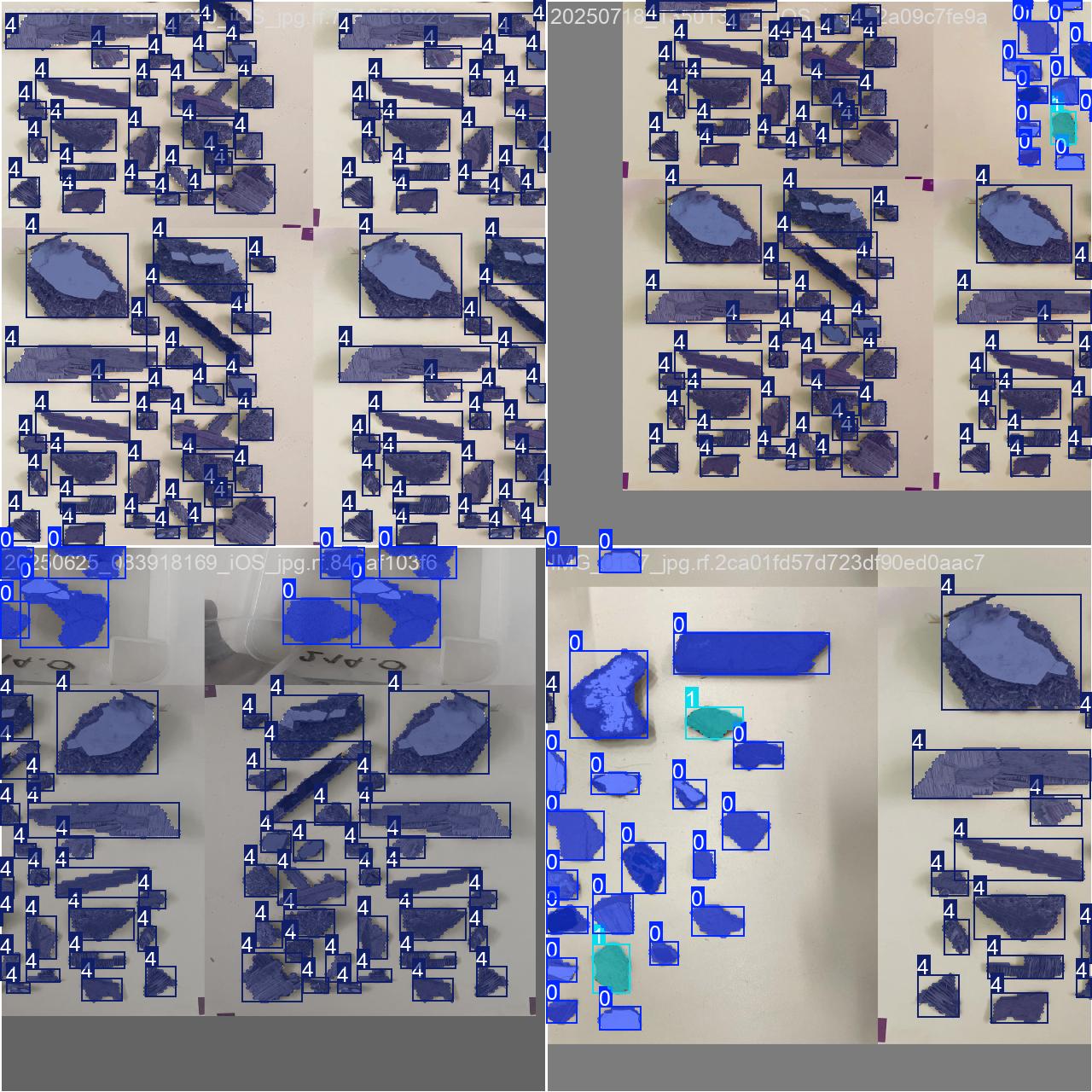
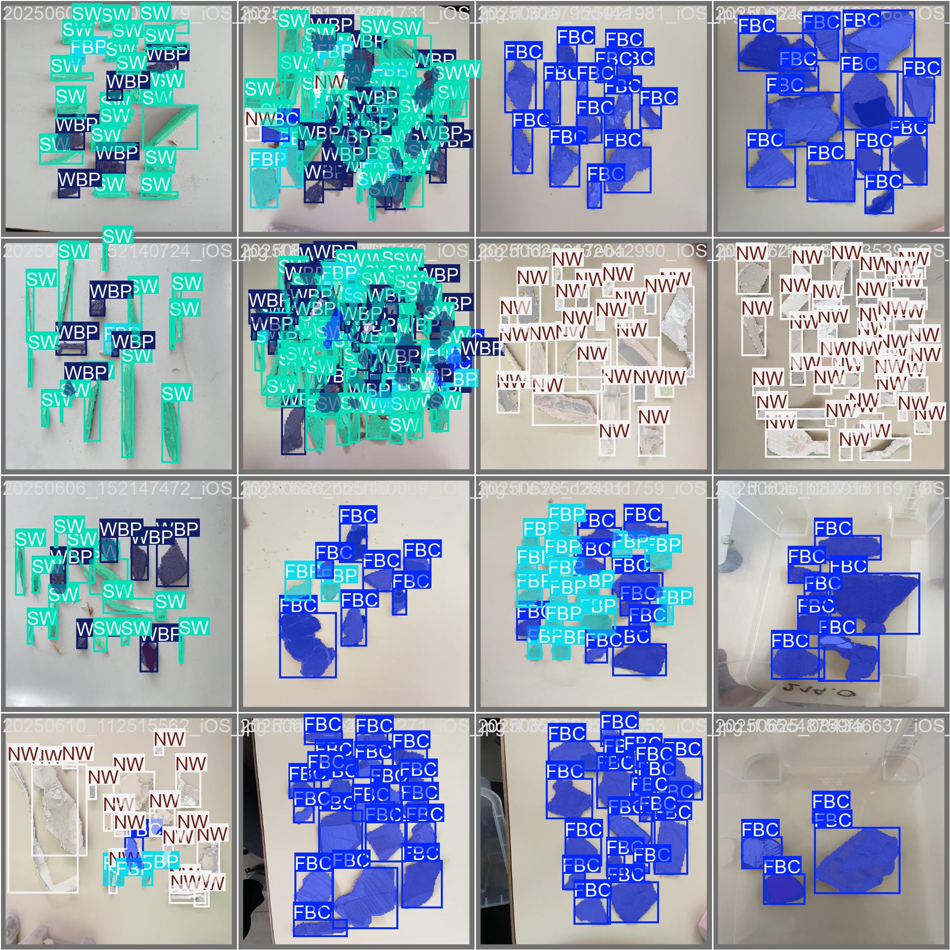
Sample outputs from the OSITY model showing detection and classification results.

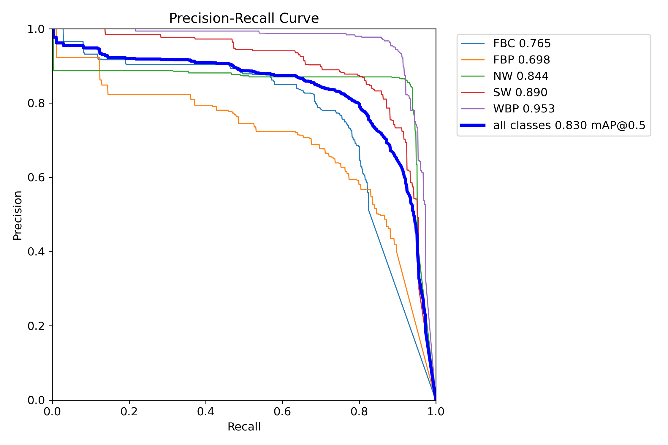
Validation Output - mAP Metrics

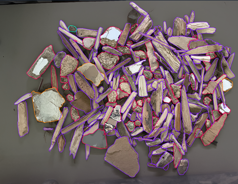
Data Annotation with Roboflow

Training Batch Sample

Validation Batch with Labels

Acknowledgments

I want to extend my thanks and appreciation to Prof. Mark Irle, the EcoRefibre project, and École Supérieure du Bois (Nantes, France) for the wonderful opportunity to freely explore this task as my personal project during my internship.

Thanks to my fellow interns for the help and insights provided during this period.

It is my hope that my work can inspire someone and can be advanced for real-world use.

— Tim Casanda Gibson

Project Links

Related Resources

Ultralytics YOLO Documentation — docs.ultralytics.com
Roboflow Universe — universe.roboflow.com

Timeline: 1 month (July 2025)

Role: Research Intern - Deep Learning Engineer

GitHub Dataset